A_B Test

Publish Date: 2019-12-22

Author: Naixin Zhang

Word Count: 2.5k

Read Times: 15 Min

Read Count:

Main script to perform an A/B experiment using simulated data

Modules: N/A
Author: Cornelia Ilin
Email: cilin@wisc.edu
Date created: Oct 13, 2019

Citations (online sources):

[1] info on Bernoulli and Binomial Random Variables, as well as Sampling Distribution of Sample Proportions
https://www.khanacademy.org/math/ap-statistics/sampling-distribution-ap/sampling-distribution-proportion/v/sampling-distribution-of-sample-proportion-part-1
[2] info on hypothesis test for sample proportions
https://www.khanacademy.org/math/ap-statistics/two-sample-inference/two-sample-z-test-proportions/v/hypothesis-test-for-difference-in-proportions-example
[3] Intro to power in significance tests
https://www.khanacademy.org/math/ap-statistics/tests-significance-ap/error-probabilities-power/v/introduction-to-power-in-significance-tests
[4] The math behind A/B testing with example code
https://towardsdatascience.com/the-math-behind-a-b-testing-with-example-code-part-1-of-2-7be752e1d06f
[5] Udacity/Google course on A/B testing
https://classroom.udacity.com/courses/ud257/lessons/4028708543/concepts/39546791500923

Citations (persons): n/a

Step 1: Define functions

def z_val(sig_level, power = False):
    """ A function that returns the z-value for given significance or power level
    param sig_level: indicates the significance level, i.e. the probability to commit a type I error
    return: z_onetail, z_twotail_minus, z_twotail_plus, z_power
    """
    # draw normal distribution with mean = 0 and se = 1 (standardized random variable)
    z_dist = scs.norm(0,1)

    # define alpha
    alpha = sig_level

    # find the value of z for which the cdf = 1 - alpha
    z_onetail = z_dist.ppf(1-alpha)

    # find the value of z for which the cdf = alpha/2, and the cdf = 1-alpha/2
    z_twotail_left = z_dist.ppf(alpha/2)
    z_twotail_right = z_dist.ppf(1 - alpha/2)

    # find the value of z for which the cdf = power
    if power:
        power_val = float(input("Introduce the desired level of power: "))
        z_power = round(z_dist.ppf(power_val), 3)
    else:
        z_power = "n/a"

    return (z_onetail, z_twotail_left, z_twotail_right, z_power)

def z_distribution(sig_level):
    """ A function that plots the distribution of the standardized random variable z
    param sig_level: indicates the significance level, i.e. the probability to commit a type I error
    return: none
    """

    # draw normal distribution with mean = 0 and se = 1 (standardized random variable)
    z_dist = scs.norm(0,1)

    # define values for x and y axes
    x = np.linspace(z_dist.ppf(0.01), z_dist.ppf(0.99), 100)
    y = z_dist.pdf(x)

    # define alpha
    alpha = sig_level

    # define arrow propoerties (used for annotations in figure)
    arrow_properties = {
        'facecolor': 'black',
        'shrink': 0.1,
        'headlength': 5,
        'width': 1
    }

    ## plot 1, one-tailed test
    plt.subplot(2,1,1).set_title("Distribution of z_statistic with one-tail test")
    lines = plt.plot(x, y)
    #plt.title('The distribution of the z-statistic')
    plt.ylabel("pdf")

    # find confidence levels, find the value of z for which the cdf = 1 - alpha
    z_onetail = z_val(alpha)[0]

    # add fill
    plt.fill_between(x, 0, y, color = "green", where = (x >= z_onetail))

    # add annotation
    annotation = plt.annotate('\u03B1 = 0.05',
                 xy = (1.98, 0.12),
                 xytext = (1.98, 0.20),
                 arrowprops = arrow_properties)


    ## plot 2, two-tailed test
    plt.subplot(2,1,2).set_title("Distribution of z_statistic with two-tail test")
    lines = plt.plot(x, y)
    plt.ylabel("pdf")
    plt.xlabel("z value")

    # find confidence levels, find the value of z for which the cdf = alpha/2, and the cdf = 1-alpha/2
    z_twotail_left = z_val(alpha)[1]
    z_twotail_right = z_val(alpha)[2]

    # add fill
    plt.fill_between(x, 0, y, color = "green", where = (x <= z_twotail_left))
    plt.fill_between(x, 0, y, color = "green", where = (x >= z_twotail_right))

    # add annotation
    annotation = plt.annotate('\u03B1 = 0.025',
                 xy = (-2.2, 0.12),
                 xytext = (-2.2, 0.20),
                 arrowprops = arrow_properties)

    annotation = plt.annotate('\u03B1 = 0.025',
                 xy = (2.2, 0.12),
                 xytext = (2.2, 0.20),
                 arrowprops = arrow_properties)

    plt.tight_layout() # adds more space between subplots

    print("z value for one-tail test = ", round(z_onetail, 3))
    print("z value for one-tail test = +-", round(z_twotail_right, 3))

def d_distribution(alpha = False, beta = False, power = False, onetail = True):
    """ A function that plots the d_distribution
    param alfa: colors the alpha region(s) when True, i.e. P(reject H0 | H0 is true) 
    param beta: computes and colors the beta region when True, i.e. P(accept H0 | H0 is false)
    param power: computes and color the power region when True, i.e. P(reject H0 | H0 is false)
    param onetail: sets test to one-tail when True
    return: none

    Note that under H0: d = 0, under Ha: d = d_hat 
    """

    # define values for the x axis
    #x = np.linspace(-0.08, 0.08, 100)
    x = np.linspace(-12 * se_pool_hat, 12 * se_pool_hat, 1000)

    # generate distribution under H0; d ~ N(0, SE_pool)
    d_dist_0 = scs.norm(0, se_pool_hat).pdf(x) 

    # generate distribution under Ha: d ~ N(d_hat, SE_pool)
    d_dist_a = scs.norm(d_hat, se_pool_hat).pdf(x)

    # plot d_dist_0, d_dist_a
    plt.subplots(figsize=(12, 6))
    lines = plt.plot(x, d_dist_0, label = "d_dist under H0")
    lines = plt.plot(x, d_dist_a, label = "d_dist under Ha")

    # add title, axis labels, and legend
    plt.title("Distribution of d under H0 and Ha")
    plt.legend()
    plt.xlabel('d value')
    plt.ylabel('pdf')

    # draw confidence intervals under H0
    # remeber ci = d +- z*se_pool, under H0: d = 0
    # for alpha = 0.05, z_onetail = 1.65, z_twotail_left = -1.96, z_twotail_right = 1.96 (see output z_dist() function)
    if onetail:
        ci_right = 0 + 1.65 * se_pool_hat
        plt.axvline(x = ci_right, linestyle = "--", color = "grey")
    else:
        ci_right = 0 + 1.96 * se_pool_hat
        ci_left = 0 - 1.96 * se_pool_hat
        plt.axvline(x = ci_left, linestyle = "--", color = "grey")
        plt.axvline(x = ci_right, linestyle = "--", color = "grey")


    # compute alpha
    # alpha = the area under H0, to the left of ci_left and to the right of ci_right
    if alpha:
        print("Green shaded area: H0 is false")
        if onetail:
            plt.fill_between(x, 0, d_dist_0, color = "olivedrab", where = (x > ci_right))
        else:
            plt.fill_between(x, 0, d_dist_0, color = "olivedrab", where = (x < ci_left))
            plt.fill_between(x, 0, d_dist_0, color = "olivedrab", where = (x > ci_right))


    # compute beta
    # beta = the area under Ha, to the left of ci_right
    if beta:
        beta_val = scs.norm(d_hat, se_pool_hat).cdf(ci_right) #finds the P(d < ci_right) under Ha
        print("Beta =", round(beta_val,3))
        print("Yelolw shaded area: Type II error area: P(accept H0|H0 is false)")
        plt.fill_between(x, 0, d_dist_a, color = "goldenrod", where = (x < ci_right))   

    # compute power
    # power = 1 - beta = the area under Ha, to the right of ci_right
    if power:
        power = 1 - scs.norm(d_hat, se_pool_hat).cdf(ci_right) #finds the P(d >= ci_right) = 1 - P (d < ci_right) under Ha
        print("Power =", round(power,3))
        print("Blue shaded area: Power = 1- Beta, P(reject H0|H0 is false)")

        plt.fill_between(x, 0, d_dist_a, color = "steelblue", where = (x > ci_right))

Step 2: Import required packages

import scipy.stats as scs
import pandas as pd
import numpy as np
import matplotlib.pyplot as plt
import random
%matplotlib inline

Step 3: Define the A/B experiment

Assume that facebook.com/business runs an A/B test to see if changing the color of the “create an ad” button, increases the click-thorugh probability.

Let’s assume that the structure of the facebook.com/business website is as follows: [1] a homepage that includes the “create an ad” button; if create an ad is chosen, then [2] a webpage to “create new account”, and if new account is created, then [3] a webpage to buy adds.

To run the A/B experiement, the engineers at facebook.com/business create two versions of the homepage. One where the “create an ad” button is orange (existing version), and one where it is blue (experimental version). The former is served to the control users, and the later to the users in the treatment group.

Unfortunately, we don’t have this data available, so we will first need to generate it.

We assume that the total number of users that participate in the A/B experiement is 2000, equally devided between the control and treated groups. This means that the probability to be assigned to either the treatment or control group is 0.5.

Step 4: Generate toy data

Notations:

group A = control patients
group B = treated patients
p_c = click-though probability for the control group
p_t = click-thorugh probability for the treated group

Step 4.1: Set seed

random.seed(1234)

Step 4.2: Create user_group column

(with values A and B)

# draw from Bernoulli distribution
user_group = scs.bernoulli.rvs(p = 0.4, size = 10000).tolist()

# rename values, such that 0 = A and 1 = B; keep track of the length of group A and B
len_A = 0
len_B = 0
for index, val in enumerate(user_group): 
    if val == 0:
        user_group[index] = "A"
        len_A += 1
    else:
        user_group[index] = "B"
        len_B += 1

Step 4.3: Create user_click column

(= 1 if a unique user clicked “create an ad” at least once)

# first define the desired p_c and p_t, assuming p_t > p_c
p_c = 0.10
p_t = 0.12

# draw user_click column from Bernoulli distribution for both group A and B
user_click_A = scs.bernoulli.rvs(p_c, size = len_A).tolist()
user_click_B = scs.bernoulli.rvs(p_t, size = len_B).tolist()

Step 4.4 Combine user_group and user_click columns

create a dataframe

# merge the two columns
user_click = []
index_A = 0
index_B = 0
for index, val in enumerate(user_group):
    if val == "A":
        user_click.append(user_click_A[index_A])
        index_A += 1
    else:
        user_click.append(user_click_B[index_B])
        index_B += 1

# create dataframe        
data = pd.DataFrame({"user_group": user_group, "user_click": user_click})

# print the first five rows:
data.head(5)

	user_group	user_click
0	B	0
1	B	0
2	B	1
3	A	0
4	A	0

Step 5: Summary statistics

We assume our toy data is the real data of facebook.com/business‘ experiment

Notation:

n_c = sample size control group
n_t = sample size treated group
x_c = number of users in the control group who click “create an ad”
x_t = number of users in the treated group who click “create an ad”
p_c_hat = estimated click-thorugh propbability of control group
p_t_hat = estimated click-thorugh probability of treated group

Step 5.1: Sample sizes

n_c = len_A
n_t = len_B
print("n_c =", n_c, end = "\n")
print("n_t =", n_t, end = "")

n_c = 6038
n_t = 3962

Step 5.2: Sum of user_click by group

x_c = 0
x_t = 0
for ind in data.index:
    if data["user_group"][ind] == "A" and data["user_click"][ind] == 1:
         x_c += 1
    if data["user_group"][ind] == "B" and data["user_click"][ind] == 1:
         x_t += 1

print("x_c = ", x_c, end = "\n")
print("x_t = ", x_t, end = "")

x_c =  605
x_t =  471

Step 5.3: Click-thourgh probability by group

Def: click-thorugh probability = unique users who click / unique total users
We can think of the click-through probability as being the sample proportion

p_c_hat = x_c/n_c
p_t_hat = x_t/n_t
print("p_c_hat = ", round(p_c_hat, 2), end = "\n")
print("p_t_hat = ", round(p_t_hat, 2), end = "")

p_c_hat =  0.1
p_t_hat =  0.12

Step 6: Hypothesis testing

We want to see if chaging the color of the “create an ad” has any statistically significant effects on the click-through probability.
Remember that “create an ad” button is orange for the control gorup, and blue for the the treated group.

Our hypothesis is as follows:
H0: p_c = p_t, in other words p_c - p_t = 0
Ha: p_t - p_c != 0 (try both one tail and two tail test)

Let:
d = p_c - p_t
alpha = P(reject H0 | H0 is true)
beta = P(accept H0 | H0 is false)
power = 1 - beta = P(reject H0 | H0 is false)

To test the hypthesis we construct the z_statistic ~ N(0, 1)

Step 6.1 Compute the z_statistic

We assume the followings:

H0 is true
random variables
iid

Then,
z = (p_t_hat - p_c_hat) - 0/ SE(p_t_hat - p_c_hat)

Note:

For a Bernoulli random variable: mean = p; variance = p(1-p); se = sqrt(p(1-p))
For Binomial random variable: mean = n p; variance = n p(1-p) = sqrt(n * (p(1-p))
Under the Central Limit Theorem, as the number of samples increases, the distribution of the sample proportion means (p_hat), will be ~ N(p, sqrt(p(1-p)/n))

Thus,
se(p_t_hat - p_c_hat) = sqrt(p_t_hat(1-p_t_hat)/n_t) + sqrt(p_c_hat(1-p_c_hat)/n_c)

Note:

cov(p_t_hat, p_c_hat) = 0 due to iid assumption.
because we assume that H0 is true (p_t = p_c), then we can compute SE_pool

Thus,
se_pool = sqrt(p_pool_hat(1-p_pool_hat) * (1/n_t + 1/n_c)
where,
p_pool_hat = (x_c + x_t)/(n_c + n_t)

# compute d = p_t_hat - p_c_hat
d_hat = p_t_hat - p_c_hat
print("d_hat =", round(d_hat, 2))

d_hat = 0.02

# compute p_pool_hat
p_pool_hat = (x_c + x_t)/(n_c + n_t)
print("p_pool_hat = ", p_pool_hat)

p_pool_hat =  0.1076

# compute se_pool_hat
se_pool_hat = np.sqrt(p_pool_hat * (1-p_pool_hat) * (1/n_c + 1/n_t))
print("se_pool_hat = ", round(se_pool_hat, 2))

se_pool_hat =  0.01

# compute the z-statistic
z_statistic = d_hat/se_pool_hat
print("z_statistic =", round(z_statistic, 2))
print("Remeber that the z-statistic is ~ N(0, 1)")

z_statistic = 2.95
Remeber that the z-statistic is ~ N(0, 1)

Step 6.2: Find p_val. Test if H0 is true

Define p_val:

if one-tailed test: p_val = P(Z >= z) = 1 - P(Z < z)
if two-tailed test: p_val = P(Z <= -z or Z >= z) = 1 - P(-z < Z < z) = 1- [P(Z < z) - P (Z < -z)]

For a one-tailed test:

if p_val > alpha, accept H0
if p_val < alpha, reject H0

For a two-tailed test:

if p_val > alpha/2, accept H0
if p_val < alpha/2, reject H0

# print message
accept = "Accept H0. p_val > alpha\n"
reject = "Reject H0. p_val < alpha\n"

# z_distribution
z_dist = scs.norm(0,1)

# alpha level
alpha = 0.05

## one-tailed test, find P(Z < z_statistic) and then compute p_val
cdf_onetail = z_dist.cdf(z_statistic)
p_val_onetail = 1 - cdf_onetail
print("one-tail test: p_val = ", round(p_val_onetail, 4), end = "\n")

if p_val_onetail < alpha:
    print(reject)
else:
    print(accept)


## two_tailed test, find P (Z < z) - P (Z < -z), then compute p_val
cdf_twotail = z_dist.cdf(z_statistic) - z_dist.cdf(-z_statistic)
p_val_twotail = 1 - cdf_twotail
print("two-tailed test: p_val = ", round(p_val_twotail, 4), end = "\n")

if p_val_twotail < alpha:
    print(reject)
else:
    print(accept)

one-tail test: p_val =  0.0016
Reject H0. p_val < alpha

two-tailed test: p_val =  0.0032
Reject H0. p_val < alpha

Step 6.3: Plot the distribution of d under H0 and Ha

d_distribution(alpha = True)

Green shaded area: H0 is false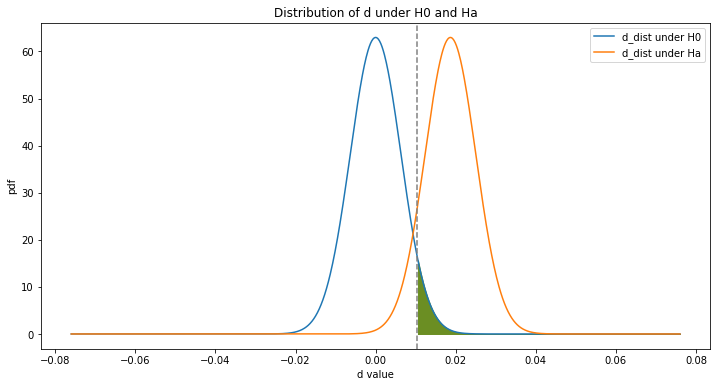

png

d_distribution(beta = True)

Beta = 0.097
Yelolw shaded area: Type II error area: P(accept H0|H0 is false)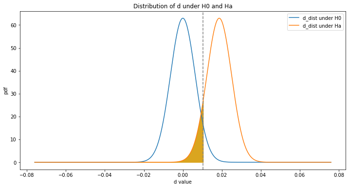

png

d_distribution(power = True)

Power = 0.903
Blue shaded area: Power = 1- Beta, P(reject H0|H0 is false)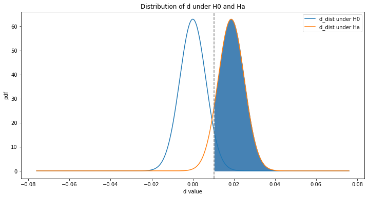

png

Step 7: Find appropiate sample size for A/B test

Note: user introduces desired beta, power, alpha, one-tail or two-tail test parameters

# define beta, power, and alpha
beta = 0.2
power = 1 - beta
alpha = 0.05
one_tail = False

# find the value of z that corresponds to the value of the power level (user input required)
z_power = z_val(alpha, power = True)[3]
print("The value of the z statistics for this level of power is", z_power)

# find the value of z that corresponds to the value of alpha
if one_tail:
    z_alpha = z_val(alpha)[0]
else:
    z_alpha = z_val(alpha)[2]

# find sample size
n = 2 * p_pool_hat * (1- p_pool_hat)*(z_power + z_alpha)**2 * (1/(p_t_hat - p_c_hat)**2)

print("The sample size needed for the parameters listed above =", round(n,2))

Introduce the desired level of power: 0.8
The value of the z statistics for this level of power is 0.842
The sample size needed for the parameters listed above = 4320.61

KPI dashboard

This is my kPI dashboard making by Excel. I learned it from Udemy https://www.udemy.com/course/excel-dashboards-reports/

2020-01-02 EXCEL

DashBoard

CS301_Proj10

CS301_Proj10IntroductionFor your final CS 301 project, you’re going to analyze the whole world! Specifically, you’re goi

2019-12-15 CS301Proj

CS301 Data Programming I