Background:
This notebook aims to build a machine learning model that predicts the probability that the first transaction of a new user is fraudulent.
Specifically, we want to solve these problems:
- for each user, determine her country based on the numeric IP address
- build model predict whether an activity is fraudulent or not.
- for a user perspective, what kind of user are more likely to be classified at risk? what are their characteristics?
- from a product perspective, how would you use it? what kind of different user experiences would you build based on the model output?
This notebook covers:
- feature engineering
- use H20 to predict fraudulent.
import bisect
import numpy as np
import pandas as pd
from sklearn.tree import DecisionTreeClassifier,export_graphviz
from sklearn.model_selection import  train_test_split
from sklearn.metrics import accuracy_score,classification_report,roc_curve
import xgboost as xgb

import matplotlib.pyplot as plt
plt.style.use('ggplot')
%matplotlib inline
import  warnings
warnings.simplefilter('ignore')

import seaborn as sns
import matplotlib.pyplot as plt
from sklearn.metrics import auc, roc_curve, classification_report

import h2o
from h2o.frame import H2OFrame
from h2o.estimators.random_forest import H2ORandomForestEstimator

%matplotlib inline
For each user, determine her country based on the numeric IP address.
data = pd.read_csv('Fraud_Data.csv', parse_dates=['signup_time', 'purchase_time'])

data.info()
<class 'pandas.core.frame.DataFrame'>
RangeIndex: 151112 entries, 0 to 151111
Data columns (total 11 columns):
user_id           151112 non-null int64
signup_time       151112 non-null datetime64[ns]
purchase_time     151112 non-null datetime64[ns]
purchase_value    151112 non-null int64
device_id         151112 non-null object
source            151112 non-null object
browser           151112 non-null object
sex               151112 non-null object
age               151112 non-null int64
ip_address        151112 non-null float64
class             151112 non-null int64
dtypes: datetime64[ns](2), float64(1), int64(4), object(4)
memory usage: 12.7+ MB
data.shape[0] == data['user_id'].nunique()
True
data.head()
|
user_id |
signup_time |
purchase_time |
purchase_value |
device_id |
source |
browser |
sex |
age |
ip_address |
class |
| 0 |
22058 |
2015-02-24 22:55:49 |
2015-04-18 02:47:11 |
34 |
QVPSPJUOCKZAR |
SEO |
Chrome |
M |
39 |
7.327584e+08 |
0 |
| 1 |
333320 |
2015-06-07 20:39:50 |
2015-06-08 01:38:54 |
16 |
EOGFQPIZPYXFZ |
Ads |
Chrome |
F |
53 |
3.503114e+08 |
0 |
| 2 |
1359 |
2015-01-01 18:52:44 |
2015-01-01 18:52:45 |
15 |
YSSKYOSJHPPLJ |
SEO |
Opera |
M |
53 |
2.621474e+09 |
1 |
| 3 |
150084 |
2015-04-28 21:13:25 |
2015-05-04 13:54:50 |
44 |
ATGTXKYKUDUQN |
SEO |
Safari |
M |
41 |
3.840542e+09 |
0 |
| 4 |
221365 |
2015-07-21 07:09:52 |
2015-09-09 18:40:53 |
39 |
NAUITBZFJKHWW |
Ads |
Safari |
M |
45 |
4.155831e+08 |
0 |
address2country = pd.read_csv('IpAddress_to_Country.csv')
address2country.head()
|
lower_bound_ip_address |
upper_bound_ip_address |
country |
| 0 |
16777216.0 |
16777471 |
Australia |
| 1 |
16777472.0 |
16777727 |
China |
| 2 |
16777728.0 |
16778239 |
China |
| 3 |
16778240.0 |
16779263 |
Australia |
| 4 |
16779264.0 |
16781311 |
China |
countries = []
for i in range(len(data)):
    ip_address = data.loc[i, 'ip_address']
    tmp = address2country[(address2country['lower_bound_ip_address'] <= ip_address) &
                          (address2country['upper_bound_ip_address'] >= ip_address)]
    if len(tmp) == 1:
        countries.append(tmp['country'].values[0])
    else:
        countries.append('NA')

data['country'] = countries

data.head()
|
user_id |
signup_time |
purchase_time |
purchase_value |
device_id |
source |
browser |
sex |
age |
ip_address |
class |
country |
| 0 |
22058 |
2015-02-24 22:55:49 |
2015-04-18 02:47:11 |
34 |
QVPSPJUOCKZAR |
SEO |
Chrome |
M |
39 |
7.327584e+08 |
0 |
Japan |
| 1 |
333320 |
2015-06-07 20:39:50 |
2015-06-08 01:38:54 |
16 |
EOGFQPIZPYXFZ |
Ads |
Chrome |
F |
53 |
3.503114e+08 |
0 |
United States |
| 2 |
1359 |
2015-01-01 18:52:44 |
2015-01-01 18:52:45 |
15 |
YSSKYOSJHPPLJ |
SEO |
Opera |
M |
53 |
2.621474e+09 |
1 |
United States |
| 3 |
150084 |
2015-04-28 21:13:25 |
2015-05-04 13:54:50 |
44 |
ATGTXKYKUDUQN |
SEO |
Safari |
M |
41 |
3.840542e+09 |
0 |
NA |
| 4 |
221365 |
2015-07-21 07:09:52 |
2015-09-09 18:40:53 |
39 |
NAUITBZFJKHWW |
Ads |
Safari |
M |
45 |
4.155831e+08 |
0 |
United States |
Feature Engineering
- Time difference between sign-up time and purchase time
- If the device id is unique or certain users are sharing the same device (many different user ids using the same device could be an indicator of fake accounts)
- Same for the ip address. Many different users having the same ip address could be an indicator of fake accounts
- Usual week of the year and day of the week from time variables
time_diff = data['purchase_time'] - data['signup_time']
time_diff = time_diff.apply(lambda x: x.seconds)
data['time_diff'] = time_diff
data.head()
|
user_id |
signup_time |
purchase_time |
purchase_value |
device_id |
source |
browser |
sex |
age |
ip_address |
class |
country |
time_diff |
| 0 |
22058 |
2015-02-24 22:55:49 |
2015-04-18 02:47:11 |
34 |
QVPSPJUOCKZAR |
SEO |
Chrome |
M |
39 |
7.327584e+08 |
0 |
Japan |
13882 |
| 1 |
333320 |
2015-06-07 20:39:50 |
2015-06-08 01:38:54 |
16 |
EOGFQPIZPYXFZ |
Ads |
Chrome |
F |
53 |
3.503114e+08 |
0 |
United States |
17944 |
| 2 |
1359 |
2015-01-01 18:52:44 |
2015-01-01 18:52:45 |
15 |
YSSKYOSJHPPLJ |
SEO |
Opera |
M |
53 |
2.621474e+09 |
1 |
United States |
1 |
| 3 |
150084 |
2015-04-28 21:13:25 |
2015-05-04 13:54:50 |
44 |
ATGTXKYKUDUQN |
SEO |
Safari |
M |
41 |
3.840542e+09 |
0 |
NA |
60085 |
| 4 |
221365 |
2015-07-21 07:09:52 |
2015-09-09 18:40:53 |
39 |
NAUITBZFJKHWW |
Ads |
Safari |
M |
45 |
4.155831e+08 |
0 |
United States |
41461 |
device_num = data[['user_id', 'device_id']].groupby('device_id').count().reset_index()
device_num = device_num.rename(columns={'user_id': 'device_num'})
data = data.merge(device_num, how='left', on='device_id')
data.head()
|
user_id |
signup_time |
purchase_time |
purchase_value |
device_id |
source |
browser |
sex |
age |
ip_address |
class |
country |
time_diff |
device_num |
| 0 |
22058 |
2015-02-24 22:55:49 |
2015-04-18 02:47:11 |
34 |
QVPSPJUOCKZAR |
SEO |
Chrome |
M |
39 |
7.327584e+08 |
0 |
Japan |
13882 |
1 |
| 1 |
333320 |
2015-06-07 20:39:50 |
2015-06-08 01:38:54 |
16 |
EOGFQPIZPYXFZ |
Ads |
Chrome |
F |
53 |
3.503114e+08 |
0 |
United States |
17944 |
1 |
| 2 |
1359 |
2015-01-01 18:52:44 |
2015-01-01 18:52:45 |
15 |
YSSKYOSJHPPLJ |
SEO |
Opera |
M |
53 |
2.621474e+09 |
1 |
United States |
1 |
12 |
| 3 |
150084 |
2015-04-28 21:13:25 |
2015-05-04 13:54:50 |
44 |
ATGTXKYKUDUQN |
SEO |
Safari |
M |
41 |
3.840542e+09 |
0 |
NA |
60085 |
1 |
| 4 |
221365 |
2015-07-21 07:09:52 |
2015-09-09 18:40:53 |
39 |
NAUITBZFJKHWW |
Ads |
Safari |
M |
45 |
4.155831e+08 |
0 |
United States |
41461 |
1 |
ip_num = data[['user_id', 'ip_address']].groupby('ip_address').count().reset_index()
ip_num = ip_num.rename(columns={'user_id': 'ip_num'})
data = data.merge(ip_num, how='left', on='ip_address')
data.head()
|
user_id |
signup_time |
purchase_time |
purchase_value |
device_id |
source |
browser |
sex |
age |
ip_address |
class |
country |
time_diff |
device_num |
ip_num |
| 0 |
22058 |
2015-02-24 22:55:49 |
2015-04-18 02:47:11 |
34 |
QVPSPJUOCKZAR |
SEO |
Chrome |
M |
39 |
7.327584e+08 |
0 |
Japan |
13882 |
1 |
1 |
| 1 |
333320 |
2015-06-07 20:39:50 |
2015-06-08 01:38:54 |
16 |
EOGFQPIZPYXFZ |
Ads |
Chrome |
F |
53 |
3.503114e+08 |
0 |
United States |
17944 |
1 |
1 |
| 2 |
1359 |
2015-01-01 18:52:44 |
2015-01-01 18:52:45 |
15 |
YSSKYOSJHPPLJ |
SEO |
Opera |
M |
53 |
2.621474e+09 |
1 |
United States |
1 |
12 |
12 |
| 3 |
150084 |
2015-04-28 21:13:25 |
2015-05-04 13:54:50 |
44 |
ATGTXKYKUDUQN |
SEO |
Safari |
M |
41 |
3.840542e+09 |
0 |
NA |
60085 |
1 |
1 |
| 4 |
221365 |
2015-07-21 07:09:52 |
2015-09-09 18:40:53 |
39 |
NAUITBZFJKHWW |
Ads |
Safari |
M |
45 |
4.155831e+08 |
0 |
United States |
41461 |
1 |
1 |
data['signup_day'] = data['signup_time'].apply(lambda x: x.dayofweek)
data['signup_week'] = data['signup_time'].apply(lambda x: x.week)
data['purchase_day'] = data['purchase_time'].apply(lambda x: x.dayofweek)
data['purchase_week'] = data['purchase_time'].apply(lambda x: x.week)
data.head()
|
user_id |
signup_time |
purchase_time |
purchase_value |
device_id |
source |
browser |
sex |
age |
ip_address |
class |
country |
time_diff |
device_num |
ip_num |
signup_day |
signup_week |
purchase_day |
purchase_week |
| 0 |
22058 |
2015-02-24 22:55:49 |
2015-04-18 02:47:11 |
34 |
QVPSPJUOCKZAR |
SEO |
Chrome |
M |
39 |
7.327584e+08 |
0 |
Japan |
13882 |
1 |
1 |
1 |
9 |
5 |
16 |
| 1 |
333320 |
2015-06-07 20:39:50 |
2015-06-08 01:38:54 |
16 |
EOGFQPIZPYXFZ |
Ads |
Chrome |
F |
53 |
3.503114e+08 |
0 |
United States |
17944 |
1 |
1 |
6 |
23 |
0 |
24 |
| 2 |
1359 |
2015-01-01 18:52:44 |
2015-01-01 18:52:45 |
15 |
YSSKYOSJHPPLJ |
SEO |
Opera |
M |
53 |
2.621474e+09 |
1 |
United States |
1 |
12 |
12 |
3 |
1 |
3 |
1 |
| 3 |
150084 |
2015-04-28 21:13:25 |
2015-05-04 13:54:50 |
44 |
ATGTXKYKUDUQN |
SEO |
Safari |
M |
41 |
3.840542e+09 |
0 |
NA |
60085 |
1 |
1 |
1 |
18 |
0 |
19 |
| 4 |
221365 |
2015-07-21 07:09:52 |
2015-09-09 18:40:53 |
39 |
NAUITBZFJKHWW |
Ads |
Safari |
M |
45 |
4.155831e+08 |
0 |
United States |
41461 |
1 |
1 |
1 |
30 |
2 |
37 |
columns = ['signup_day', 'signup_week', 'purchase_day', 'purchase_week', 'purchase_value', 'source',
'browser', 'sex', 'age', 'country', 'time_diff', 'device_num', 'ip_num', 'class']
data = data[columns]
data.head()
|
signup_day |
signup_week |
purchase_day |
purchase_week |
purchase_value |
source |
browser |
sex |
age |
country |
time_diff |
device_num |
ip_num |
class |
| 0 |
1 |
9 |
5 |
16 |
34 |
SEO |
Chrome |
M |
39 |
Japan |
13882 |
1 |
1 |
0 |
| 1 |
6 |
23 |
0 |
24 |
16 |
Ads |
Chrome |
F |
53 |
United States |
17944 |
1 |
1 |
0 |
| 2 |
3 |
1 |
3 |
1 |
15 |
SEO |
Opera |
M |
53 |
United States |
1 |
12 |
12 |
1 |
| 3 |
1 |
18 |
0 |
19 |
44 |
SEO |
Safari |
M |
41 |
NA |
60085 |
1 |
1 |
0 |
| 4 |
1 |
30 |
2 |
37 |
39 |
Ads |
Safari |
M |
45 |
United States |
41461 |
1 |
1 |
0 |
Fraudulent Activity Identification
h2o.init()
h2o.remove_all()
Checking whether there is an H2O instance running at http://localhost:54321 ..... not found.
Attempting to start a local H2O server...
; Java HotSpot(TM) 64-Bit Server VM (build 25.181-b13, mixed mode)
  Starting server from C:\Users\Naixin\Anaconda3\lib\site-packages\h2o\backend\bin\h2o.jar
  Ice root: C:\Users\Naixin\AppData\Local\Temp\tmpaer_0p20
  JVM stdout: C:\Users\Naixin\AppData\Local\Temp\tmpaer_0p20\h2o_Naixin_started_from_python.out
  JVM stderr: C:\Users\Naixin\AppData\Local\Temp\tmpaer_0p20\h2o_Naixin_started_from_python.err
  Server is running at http://127.0.0.1:54321
Connecting to H2O server at http://127.0.0.1:54321 ... successful.
| H2O cluster uptime: |
03 secs |
| H2O cluster timezone: |
America/Chicago |
| H2O data parsing timezone: |
UTC |
| H2O cluster version: |
3.26.0.6 |
| H2O cluster version age: |
5 days |
| H2O cluster name: |
H2O_from_python_Naixin_uxelgu |
| H2O cluster total nodes: |
1 |
| H2O cluster free memory: |
1.747 Gb |
| H2O cluster total cores: |
0 |
| H2O cluster allowed cores: |
0 |
| H2O cluster status: |
accepting new members, healthy |
| H2O connection url: |
http://127.0.0.1:54321 |
| H2O connection proxy: |
None |
| H2O internal security: |
False |
| H2O API Extensions: |
Amazon S3, Algos, AutoML, Core V3, TargetEncoder, Core V4 |
| Python version: |
3.7.3 final |
h2o_df = H2OFrame(data)
for name in ['signup_day', 'purchase_day', 'source', 'browser', 'sex', 'country', 'class']:
h2o_df[name] = h2o_df[name].asfactor()
h2o_df.summary()
Parse progress: |█████████████████████████████████████████████████████████| 100%
| | signup_day | signup_week | purchase_day | purchase_week | purchase_value | source | browser | sex | age | country | time_diff | device_num | ip_num | class |
|---|
| type | enum | int | enum | int | int | enum | enum | enum | int | enum | int | int | int | enum |
| mins | | 1.0 | | 1.0 | 9.0 | | | | 18.0 | | 1.0 | 1.0 | 1.0 | |
| mean | | 16.50174043093866 | | 24.65857112605202 | 36.93537243898601 | | | | 33.14070358409675 | | 40942.58442744426 | 1.6843665625496351 | 1.6027185134205097 | |
| maxs | | 34.0 | | 51.0 | 154.0 | | | | 76.0 | | 86399.0 | 20.0 | 20.0 | |
| sigma | | 9.814287461798903 | | 11.651556782719481 | 18.32276214866213 | | | | 8.617733490961495 | | 26049.66190211841 | 2.616953602804173 | 2.596239527375834 | |
| zeros | | 0 | | 0 | 0 | | | | 0 | | 0 | 0 | 0 | |
| missing | 0 | 0 | 0 | 0 | 0 | 0 | 0 | 0 | 0 | 0 | 0 | 0 | 0 | 0 |
| 0 | 1 | 9.0 | 5 | 16.0 | 34.0 | SEO | Chrome | M | 39.0 | Japan | 13882.0 | 1.0 | 1.0 | 0 |
| 1 | 6 | 23.0 | 0 | 24.0 | 16.0 | Ads | Chrome | F | 53.0 | United States | 17944.0 | 1.0 | 1.0 | 0 |
| 2 | 3 | 1.0 | 3 | 1.0 | 15.0 | SEO | Opera | M | 53.0 | United States | 1.0 | 12.0 | 12.0 | 1 |
| 3 | 1 | 18.0 | 0 | 19.0 | 44.0 | SEO | Safari | M | 41.0 | NA | 60085.0 | 1.0 | 1.0 | 0 |
| 4 | 1 | 30.0 | 2 | 37.0 | 39.0 | Ads | Safari | M | 45.0 | United States | 41461.0 | 1.0 | 1.0 | 0 |
| 5 | 3 | 21.0 | 3 | 28.0 | 42.0 | Ads | Chrome | M | 18.0 | Canada | 7331.0 | 1.0 | 1.0 | 0 |
| 6 | 5 | 31.0 | 3 | 35.0 | 11.0 | Ads | Chrome | F | 19.0 | NA | 17825.0 | 1.0 | 1.0 | 0 |
| 7 | 0 | 15.0 | 0 | 22.0 | 27.0 | Ads | Opera | M | 34.0 | United States | 35129.0 | 1.0 | 1.0 | 0 |
| 8 | 1 | 17.0 | 1 | 23.0 | 30.0 | SEO | IE | F | 43.0 | China | 51800.0 | 1.0 | 1.0 | 0 |
| 9 | 6 | 4.0 | 0 | 13.0 | 62.0 | Ads | IE | M | 31.0 | United States | 18953.0 | 1.0 | 1.0 | 0 |
strat_split = h2o_df['class'].stratified_split(test_frac=0.3, seed=42)
train = h2o_df[strat_split == 'train']
test = h2o_df[strat_split == 'test']
feature = ['signup_day', 'signup_week', 'purchase_day', 'purchase_week', 'purchase_value',
'source', 'browser', 'sex', 'age', 'country', 'time_diff', 'device_num', 'ip_num']
target = 'class'
model = H2ORandomForestEstimator(balance_classes=True, ntrees=100, mtries=-1, stopping_rounds=5,
stopping_metric='auc', score_each_iteration=True, seed=42)
model.train(x=feature, y=target, training_frame=train, validation_frame=test)
drf Model Build progress: |███████████████████████████████████████████████| 100%
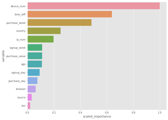
importance = model.varimp(use_pandas=True)
fig, ax = plt.subplots(figsize=(10, 8))
sns.barplot(x='scaled_importance', y='variable', data=importance)
plt.show()
train_true = train.as_data_frame()['class'].values
test_true = test.as_data_frame()['class'].values
train_pred = model.predict(train).as_data_frame()['p1'].values
test_pred = model.predict(test).as_data_frame()['p1'].values
train_fpr, train_tpr, _ = roc_curve(train_true, train_pred)
test_fpr, test_tpr, _ = roc_curve(test_true, test_pred)
train_auc = np.round(auc(train_fpr, train_tpr), 3)
test_auc = np.round(auc(test_fpr, test_tpr), 3)
drf prediction progress: |████████████████████████████████████████████████| 100%
drf prediction progress: |████████████████████████████████████████████████| 100%
print(classification_report(y_true=test_true, y_pred=(test_pred > 0.5).astype(int)))
              precision    recall  f1-score   support

           0       0.95      1.00      0.98     41088
           1       1.00      0.53      0.69      4245

    accuracy                           0.96     45333
   macro avg       0.98      0.76      0.83     45333
weighted avg       0.96      0.96      0.95     45333
train_fpr = np.insert(train_fpr, 0, 0)
train_tpr = np.insert(train_tpr, 0, 0)
test_fpr = np.insert(test_fpr, 0, 0)
test_tpr = np.insert(test_tpr, 0, 0)

fig, ax = plt.subplots(figsize=(8, 6))
ax.plot(train_fpr, train_tpr, label='Train AUC: ' + str(train_auc))
ax.plot(test_fpr, test_tpr, label='Test AUC: ' + str(test_auc))
ax.plot(train_fpr, train_fpr, 'k--', label='Chance Curve')
ax.set_xlabel('False Positive Rate', fontsize=12)
ax.set_ylabel('True Positive Rate', fontsize=12)
ax.grid(True)
ax.legend(fontsize=12)
plt.show()
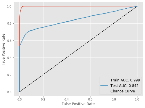
Based on the ROC, if we care about minimizing false positive, we would choose a cut-off that would give us true positive rate of ~0.5 and false positive rate almost zero (this was essentially the random forest output). However, if we care about maximizing true positive, we will have to decrease the cut-off. This way we will classify more events as “1”: some will be true ones (so true positive goes up) and many, unfortunately, will be false ones (so false positive will also go up).
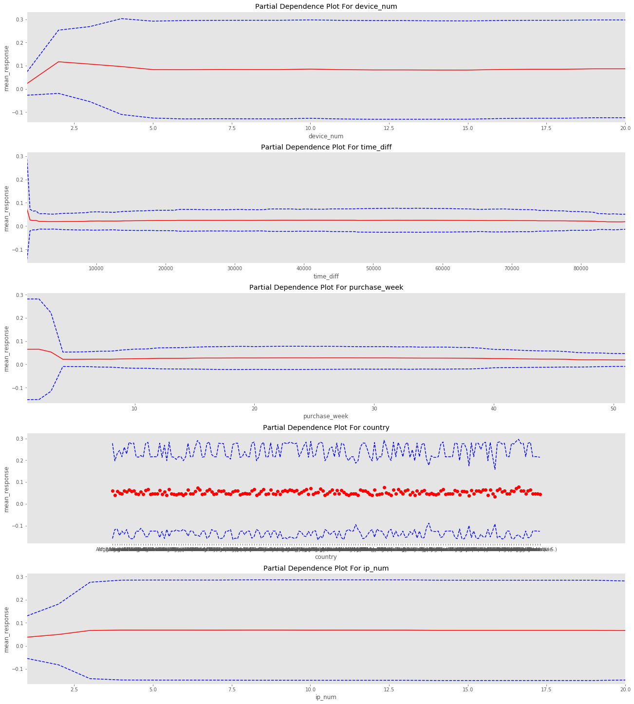
cols = ['device_num', 'time_diff', 'purchase_week', 'country', 'ip_num']
_ = model.partial_plot(data=train, cols=cols, nbins=200, figsize=(18, 20))
PartialDependencePlot progress: |█████████████████████████████████████████| 100%
h2o.cluster().shutdown()
Regarding “how to use this from a product perspective”: you now have a model that assigns to each user a probability of committing a fraud. You want to think about creating different experiences based on that. For instance:
- If predicted fraud probability < X, the user has the normal experience (the high majority should fall here)
- If X <= predicted fraud probability < Z (so the user is at risk, but not too much), you can create an additional verification step, like verify your phone number via a code sent by SMS or log in via Facebook.
- If predicted fraud probability >= Z (so here is really likely the user is trying to commit a fraud), you can tell the user his session has been put on hold, send this user info to someone who reviews it manually and either blocks the user or decides it is not a fraud so the session is resumed.
This is just an example and there are many different ways to build products around some fraud score. However, it is important because it highlights that a ML model is often really useful when it is combined with a product which is able to take advantage of its strengths and minimize its possible drawbacks (like false positives).