Take home data challenge

Publish Date: 2018-01-31

Author: Naixin Zhang

Word Count: 3.2k

Read Times: 19 Min

Read Count:

Background: This notebook aims to evaluate whether a pricing test running on the site has been successful. Specifically, we will invesigate:

Should the company sell its software for 39 or 59?
The VP of Product is interested in having a holistic view into user behavior, especially focusing on actionable insights that might increase conversion rate. What are your main ﬁndings looking at the data?
The VP of Product feels that the test has been running for too long and he should have been able to get statistically signiﬁcant results in a shorter time. Do you agree with her intuition? After how many days you would have stopped the test? Please, explain why.

Index

Load the data
Check whether test/control group is randomly splitted?
Answer question 1
Answer question 2

import numpy as np
import pandas as pd
import scipy.stats as ss
from sklearn.preprocessing import LabelEncoder
from sklearn.feature_selection import chi2,f_classif
from sklearn.tree import DecisionTreeClassifier,export_graphviz

import matplotlib.pyplot as plt
plt.style.use('ggplot')
%matplotlib inline

seed = 999

Load the data

testdata = pd.read_csv("test_results.csv",index_col="user_id")
# users contains [id,city,country,lat,long]
# and all 'country' column is USA
# I don't think users can provide useful information to the problems, so just ignore user_table.csv
# users = pd.read_csv("user_table.csv")

# some time has 60 seconds/minute, which cannot be processed by to_datetime
# if given more time, I will fix this incorrect format
# testdata["timestamp"] = pd.to_datetime(testdata.timestamp)

# rename to short names, make it easier to display
testdata.rename(columns={'operative_system':'OS'},inplace=True)

testdata.head()

	timestamp	source	device	OS	test	price	converted
user_id
604839	2015-05-08 03:38:34	ads_facebook	mobile	iOS	0	39	0
624057	2015-05-10 21:08:46	seo-google	mobile	android	0	39	0
317970	2015-04-04 15:01:23	ads-bing	mobile	android	0	39	0
685636	2015-05-07 07:26:01	direct_traffic	mobile	iOS	1	59	0
820854	2015-05-24 11:04:40	ads_facebook	web	mac	0	39	0

Check whether test and control group is randomly splitted?

X = testdata.copy()
del X['timestamp']

# to use sklearn to check feature importance, we must convert string values to numbers
src_label_encoder = LabelEncoder()
dev_label_encoder = LabelEncoder()
os_label_encoder = LabelEncoder()

X["source"] = src_label_encoder.fit_transform(testdata.source)
X["device"] = dev_label_encoder.fit_transform(testdata.device)
X["OS"] = os_label_encoder.fit_transform(testdata.OS)

X.head()

	source	device	OS	test	price	converted
user_id
604839	3	0	1	0	39	0
624057	8	0	0	0	39	0
317970	0	0	0	0	39	0
685636	5	0	1	1	59	0
820854	3	1	3	0	39	0

run Chi-Square test to see which factor impact the splitting between test/control group

colnames = ["source","device","OS"]
ch2values,pvalues = chi2(X.loc[:,colnames],X["test"])
pd.DataFrame({'chi2_value':ch2values,'pvalue':pvalues},index = colnames).sort_values(by='pvalue')

	chi2_value	pvalue
OS	83.085986	7.856065e-20
device	44.366335	2.723301e-11
source	0.924742	3.362329e-01

from above result, we know that the splitting between test/control groups aren’t random. OS and device has great impact on the split.

def calc_ratios(s):
    d = s.value_counts(normalize=True)
    d['total'] = s.shape[0]
    return d
test_ctrl_by_os = testdata.groupby('OS')['test'].apply(calc_ratios).unstack()
test_ctrl_by_os

	0	1	total
OS
android	0.643358	0.356642	74935.0
iOS	0.647934	0.352066	95465.0
linux	0.533736	0.466264	4135.0
mac	0.652422	0.347578	25085.0
other	0.647865	0.352135	16204.0
windows	0.629764	0.370236	100976.0

test_ctrl_by_os.plot(kind='bar',figsize=(15,5))

<matplotlib.axes._subplots.AxesSubplot at 0x18b2f2c8c50>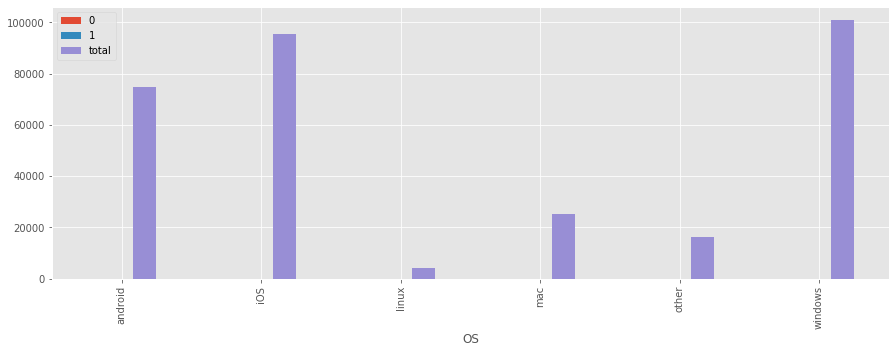

png

os_by_test_ctrl = testdata.groupby('test')['OS'].apply(lambda s: s.value_counts(normalize=True)).unstack()
os_by_test_ctrl

	windows	iOS	android	mac	other	linux
test
0	0.313678	0.305115	0.237807	0.080729	0.051784	0.010887
1	0.327729	0.294636	0.234280	0.076434	0.050021	0.016901

os_by_test_ctrl.plot(kind='bar',figsize=(15,5))

<matplotlib.axes._subplots.AxesSubplot at 0x18b2f3647f0>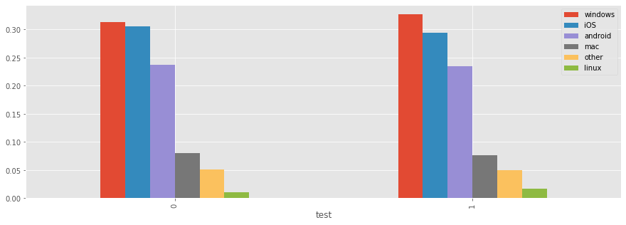

png

we can see that OS distribution in test/control groups are very different.

the experiment claim that ‘66% of the users have seen the old price (39), while a random sample of 33% users a higher price (59).’, but users from Linux don’t obey such rule, but 53% go to control group, 47% go to test group.

Answer question 1

Should the company sell its software for 39 or 59?

revenues = testdata.groupby(by="test").apply(lambda df: df.price * df.converted)
ctrl_revenues = revenues[0]
test_revenues = revenues[1]

def group_statistics(df):
    return pd.Series({'n_users': df.shape[0],
                      'convert_rate': df.converted.mean(), 
                      'mean_revenue': (df.price * df.converted).mean()})
testdata.groupby('test').apply(group_statistics)

	n_users	convert_rate	mean_revenue
test
0	202727.0	0.019904	0.776734
1	114073.0	0.015543	0.916843

we are going to perform a t-test to test whether the test group’s average revenue is higher than control group’s average revenue

H0: test group’s average revenue equal to control group’s average revenue
HA: test group’s average revenue is higher than control group’s average revenue

ttest_result = ss.ttest_ind(test_revenues,ctrl_revenues,equal_var=False)
# ttest_ind is a two tailed
# since our HA is test_mean > ctrl_mean, so we need to divide by 2
ttest_result.pvalue/2

7.703749302339191e-09

since the p-value is much smaller than 0.05 threshold, so we reject H0, and accept HA, that is, test group’s average revenue is significantly higher than control group’s average revenue.

but due to OS distribution aren’t the same between test/control groups, price isn’t the only difference between test/control groups, so we cannot contribute the increase in average revenue to price.

the experiment design fails, I cannot answer decide whether we can sell software to all users in 59 dollars. I suggest

find the reason why linux users have different representation ratio than other OS.
then run the experiment again, make sure price is the only difference between test and control group
then run t-test again, to see whether the average revenue is significantly improved.
then I can draw the conclusion.

Answer question 2

The VP of Product is interested in having a holistic view into user behavior, especially focusing on actionable insights that might increase conversion rate. What are your main ﬁndings looking at the data?

# X is the data after being transformed by LabelEncoder
X.tail()# glance the data

	source	device	OS	test	price	converted
user_id
17427	3	1	5	0	39	0
687787	5	1	5	0	39	0
618863	1	1	3	0	39	0
154636	6	0	0	0	39	0
832372	3	0	0	1	59	0

Chi-Square test

I first run Chi-Square test to see which feature greatly impact converted or not

colnames = ["source","device","OS",'price']
ch2values,pvalues = chi2(X.loc[:,colnames],X["converted"])
pd.DataFrame({'chi2_value':ch2values,'pvalue':pvalues},index = colnames).sort_values(by='pvalue')

	chi2_value	pvalue
price	150.992849	1.051844e-34
OS	7.642955	5.699447e-03
source	2.373391	1.234187e-01
device	0.729490	3.930485e-01

Chi-Square test tells us,

Price and OS are two main factor which impact converted or not.
Source and Device don’t impact conversion rate that much.

How price affects conversion?

converted_by_price= testdata.groupby("price")['converted'].apply(lambda s: s.value_counts(normalize=True)).unstack()
converted_by_price

	0	1
price
39	0.980111	0.019889
59	0.984430	0.015570

Users see 59 dollar has lower conversion rate than users see 39 dollars.

How OS affects conversion?

converted_by_os = testdata.groupby("OS")['converted'].apply(lambda s: s.value_counts(normalize=True)).unstack()
converted_by_os.sort_values(by=1,ascending=False)

	0	1
OS
mac	0.976002	0.023998
iOS	0.977678	0.022322
windows	0.983045	0.016955
android	0.985067	0.014933
other	0.987040	0.012960
linux	0.991778	0.008222

os_by_converted = testdata.groupby("converted")['OS'].apply(lambda s: s.value_counts(normalize=True)).unstack()
os_by_converted

	android	iOS	linux	mac	other	windows
converted
0	0.237357	0.300117	0.013187	0.078725	0.051429	0.319185
1	0.192665	0.366908	0.005854	0.103650	0.036157	0.294766

os_by_converted.plot(kind='bar',figsize=(10,5))

<matplotlib.axes._subplots.AxesSubplot at 0x18b2f403e80>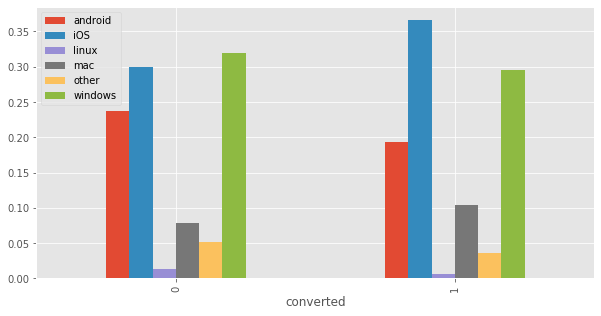

png

os_by_converted.transpose().plot(kind='bar')

<matplotlib.axes._subplots.AxesSubplot at 0x18b2f521668>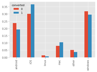

png

from above result, we can see

Mac and iOS users have higher conversion rate than users from other OS.
Linux users have lower conversion rate than users from other OS.

Model by Decision Tree

I will build a Decision Tree to get feature importance. Since the question is asking about “actionable insight” other than a model which precisely predict converted or not, so I will just fit a shallow Decision Tree on all the data, without giving out model’s performance on test set.

testdata.sample(10)# glance the data

	timestamp	source	device	OS	test	price	converted
user_id
523888	2015-04-24 11:44:22	ads-yahoo	mobile	iOS	1	59	0
42215	2015-05-22 05:48:48	ads-yahoo	mobile	iOS	1	59	0
747474	2015-04-04 03:09:29	ads_facebook	mobile	iOS	1	59	0
340105	2015-04-30 09:43:25	direct_traffic	web	linux	0	39	0
43494	2015-03-06 08:12:10	seo-bing	mobile	iOS	0	39	0
588932	2015-04-10 10:28:60	ads-yahoo	mobile	other	0	39	0
729102	2015-04-20 09:41:18	ads_facebook	web	windows	0	39	0
949907	2015-04-19 01:32:28	direct_traffic	mobile	android	0	39	0
882247	2015-04-24 02:04:20	ads_other	mobile	android	0	39	0
489936	2015-04-10 05:52:26	ads-bing	mobile	iOS	0	39	0

X = testdata.copy()
del X['timestamp']
del X['test']

X.source.value_counts()

direct_traffic     60357
ads-google         59379
ads_facebook       53396
ads_other          29876
seo-google         23175
ads-bing           22873
seo_facebook       21205
friend_referral    20695
seo-other           9260
ads-yahoo           7583
seo-yahoo           6848
seo-bing            2153
Name: source, dtype: int64

X.device.value_counts()

mobile    186471
web       130329
Name: device, dtype: int64

X.OS.value_counts()

windows    100976
iOS         95465
android     74935
mac         25085
other       16204
linux        4135
Name: OS, dtype: int64

# One-Hot-Encoding on categorical features
X = pd.get_dummies(X)

# a categorical feature of K unique values, only need K-1 vectors
# I don't use 'drop_first' parameter in get_dummies, since it cannot specify which level to drop
del X['source_ads_other']
del X['device_web']
del X['OS_other']

X.tail()# glance the data

	price	converted	source_ads-bing	source_ads-google	source_ads-yahoo	source_ads_facebook	source_direct_traffic	source_friend_referral	source_seo-bing	source_seo-google	source_seo-other	source_seo-yahoo	source_seo_facebook	device_mobile	OS_android	OS_iOS	OS_linux	OS_mac	OS_windows
user_id
17427	39	0	0	0	0	1	0	0	0	0	0	0	0	0	0	0	0	0	1
687787	39	0	0	0	0	0	1	0	0	0	0	0	0	0	0	0	0	0	1
618863	39	0	0	1	0	0	0	0	0	0	0	0	0	0	0	0	0	1	0
154636	39	0	0	0	0	0	0	1	0	0	0	0	0	1	1	0	0	0	0
832372	59	0	0	0	0	1	0	0	0	0	0	0	0	1	1	0	0	0	0

Xtrain = X.loc[:,X.columns != 'converted']
ytrain = X.loc[:,'converted']

Xtrain.head()# glance the data

	price	source_ads-bing	source_ads-google	source_ads-yahoo	source_ads_facebook	source_direct_traffic	source_friend_referral	source_seo-bing	source_seo-google	source_seo-other	source_seo-yahoo	source_seo_facebook	device_mobile	OS_android	OS_iOS	OS_linux	OS_mac	OS_windows
user_id
604839	39	0	0	0	1	0	0	0	0	0	0	0	1	0	1	0	0	0
624057	39	0	0	0	0	0	0	0	1	0	0	0	1	1	0	0	0	0
317970	39	1	0	0	0	0	0	0	0	0	0	0	1	1	0	0	0	0
685636	59	0	0	0	0	1	0	0	0	0	0	0	1	0	1	0	0	0
820854	39	0	0	0	1	0	0	0	0	0	0	0	0	0	0	0	1	0

dt = DecisionTreeClassifier(max_depth=4)
dt.fit(Xtrain,ytrain)
export_graphviz(dt,feature_names=Xtrain.columns,proportion=True,leaves_parallel=True)

'digraph Tree {\nnode [shape=box] ;\ngraph [ranksep=equally, splines=polyline] ;\n0 [label="source_friend_referral <= 0.5\\ngini = 0.036\\nsamples = 100.0%\\nvalue = [0.982, 0.018]"] ;\n1 [label="OS_iOS <= 0.5\\ngini = 0.033\\nsamples = 93.5%\\nvalue = [0.983, 0.017]"] ;\n0 -> 1 [labeldistance=2.5, labelangle=45, headlabel="True"] ;\n2 [label="OS_mac <= 0.5\\ngini = 0.03\\nsamples = 65.3%\\nvalue = [0.985, 0.015]"] ;\n1 -> 2 ;\n3 [label="source_direct_traffic <= 0.5\\ngini = 0.028\\nsamples = 58.0%\\nvalue = [0.986, 0.014]"] ;\n2 -> 3 ;\n4 [label="gini = 0.03\\nsamples = 46.1%\\nvalue = [0.985, 0.015]"] ;\n3 -> 4 ;\n5 [label="gini = 0.02\\nsamples = 11.9%\\nvalue = [0.99, 0.01]"] ;\n3 -> 5 ;\n6 [label="source_ads-bing <= 0.5\\ngini = 0.044\\nsamples = 7.4%\\nvalue = [0.977, 0.023]"] ;\n2 -> 6 ;\n7 [label="gini = 0.046\\nsamples = 6.8%\\nvalue = [0.976, 0.024]"] ;\n6 -> 7 ;\n8 [label="gini = 0.026\\nsamples = 0.5%\\nvalue = [0.987, 0.013]"] ;\n6 -> 8 ;\n9 [label="source_ads-google <= 0.5\\ngini = 0.041\\nsamples = 28.1%\\nvalue = [0.979, 0.021]"] ;\n1 -> 9 ;\n10 [label="source_ads_facebook <= 0.5\\ngini = 0.038\\nsamples = 22.4%\\nvalue = [0.981, 0.019]"] ;\n9 -> 10 ;\n11 [label="gini = 0.035\\nsamples = 17.2%\\nvalue = [0.982, 0.018]"] ;\n10 -> 11 ;\n12 [label="gini = 0.049\\nsamples = 5.2%\\nvalue = [0.975, 0.025]"] ;\n10 -> 12 ;\n13 [label="price <= 49.0\\ngini = 0.051\\nsamples = 5.7%\\nvalue = [0.974, 0.026]"] ;\n9 -> 13 ;\n14 [label="gini = 0.051\\nsamples = 3.7%\\nvalue = [0.974, 0.026]"] ;\n13 -> 14 ;\n15 [label="gini = 0.05\\nsamples = 2.0%\\nvalue = [0.974, 0.026]"] ;\n13 -> 15 ;\n16 [label="price <= 49.0\\ngini = 0.074\\nsamples = 6.5%\\nvalue = [0.961, 0.039]"] ;\n0 -> 16 [labeldistance=2.5, labelangle=-45, headlabel="False"] ;\n17 [label="OS_iOS <= 0.5\\ngini = 0.08\\nsamples = 4.1%\\nvalue = [0.958, 0.042]"] ;\n16 -> 17 ;\n18 [label="OS_linux <= 0.5\\ngini = 0.077\\nsamples = 2.9%\\nvalue = [0.96, 0.04]"] ;\n17 -> 18 ;\n19 [label="gini = 0.077\\nsamples = 2.8%\\nvalue = [0.96, 0.04]"] ;\n18 -> 19 ;\n20 [label="gini = 0.096\\nsamples = 0.0%\\nvalue = [0.949, 0.051]"] ;\n18 -> 20 ;\n21 [label="gini = 0.086\\nsamples = 1.3%\\nvalue = [0.955, 0.045]"] ;\n17 -> 21 ;\n22 [label="OS_linux <= 0.5\\ngini = 0.065\\nsamples = 2.4%\\nvalue = [0.966, 0.034]"] ;\n16 -> 22 ;\n23 [label="OS_iOS <= 0.5\\ngini = 0.067\\nsamples = 2.3%\\nvalue = [0.965, 0.035]"] ;\n22 -> 23 ;\n24 [label="gini = 0.061\\nsamples = 1.6%\\nvalue = [0.969, 0.031]"] ;\n23 -> 24 ;\n25 [label="gini = 0.08\\nsamples = 0.7%\\nvalue = [0.958, 0.042]"] ;\n23 -> 25 ;\n26 [label="gini = 0.0\\nsamples = 0.1%\\nvalue = [1.0, 0.0]"] ;\n22 -> 26 ;\n{rank=same ; 0} ;\n{rank=same ; 1; 16} ;\n{rank=same ; 2; 9; 17; 22} ;\n{rank=same ; 3; 6; 10; 13; 18; 23} ;\n{rank=same ; 4; 5; 7; 8; 11; 12; 14; 15; 19; 20; 21; 24; 25; 26} ;\n}'

from above tree plot, we can see that, to reach the leaf node with highest conversion rate (the third leaf from right with conversion rate=0.05), the path is:

source ‘friend_referral’ = true
price < 49, i.e., price = 39
OS ‘iOS’= true

pd.Series(dt.feature_importances_,index = Xtrain.columns).sort_values(ascending=False)

source_friend_referral    0.582278
OS_iOS                    0.136605
OS_mac                    0.093907
source_direct_traffic     0.059002
source_ads_facebook       0.041034
source_ads-google         0.038543
price                     0.020118
OS_linux                  0.018002
source_ads-bing           0.010511
source_ads-yahoo          0.000000
OS_windows                0.000000
source_seo-bing           0.000000
source_seo-other          0.000000
source_seo-yahoo          0.000000
source_seo_facebook       0.000000
device_mobile             0.000000
OS_android                0.000000
source_seo-google         0.000000
dtype: float64

Actionable Insights

friend_referral, Apple user (MAC or iOS), low price are three great positive factors which improve the conversion rate
if we want to increase the price, which impacts negatively on conversion rate, we must compensate on the other two factors
- lauch special marketing program targeted to Apple users (MAC or iOS users)
- run some program which rewards user which can invite his/her friend to use our software
Linux users don’t like our software as much as users on other OS. Development team should find out the reason. For example, is there any incompatibility issue on Linux?

7-Marketing Email campaign

Background: This notebook aims to optimize the marketing campaigns. Specifically, we will achieve: - What percentage

2018-02-01 Take home data challenge

Python_Take home challenge

4-Identifying Fraudulent activities

Background: This notebook aims to build a machine learning model that predicts the probability that the first transactio

2018-01-24 Take home data challenge

Python_Take home challenge