7-Marketing Email campaign

Take home data challenge

Publish Date: 2018-02-01

Author: Naixin Zhang

Word Count: 4.5k

Read Times: 28 Min

Read Count:

Background: This notebook aims to optimize the marketing campaigns. Specifically, we will achieve: - What percentage of users opened the email? - what percentage clicked on the link within the email? - build a model to optimize in future email campaigns to maximize the probability of users who click on the link/total users who received the email. How would you test that - find interesting pattern on how the email campaign performed for different segments of users.

import itertools
import _pickle as cPickle
import numpy as np
import pandas as pd
import matplotlib.pyplot as plt
plt.style.use("ggplot")
from sklearn.feature_selection import chi2,f_classif
from sklearn.preprocessing import LabelEncoder
from sklearn.metrics import classification_report,roc_curve,precision_score,recall_score,auc,precision_recall_curve
from sklearn.model_selection import train_test_split
import xgboost as xgb

seed = 9999
plt.style.use('ggplot')
%matplotlib inline

Index

Load emails from CSV
Answer Question 1
Explore the data
Answer Question 4
Build Predictive Model
Answer question 2 and question 3’s first part
Answer question 3’s second part
Answers summary:

Load emails information from CSV file

emails = pd.read_csv("email_table.csv",index_col="email_id")

Columns:

email_id : the Id of the email that was sent. It is unique by email
email_text : there are two versions of the email: one has “long text” (i.e. has 4 paragraphs) and one has “short text” (just 2 paragraphs)
email_version : some emails were “personalized” (i.e. they had the name of the user receiving the email in the incipit, such as “Hi John,”), while some emails were “generic” (the incipit was just “Hi,”).
hour : the user local time when the email was sent.
weekday : the day when the email was sent.
user_country : the country where the user receiving the email was based. It comes from the user ip address when she created the account.
user_past_purchases : how many items in the past were bought by the user receiving the email

emails.sample(10)# view some data to get a feeling

	email_text	email_version	hour	weekday	user_country	user_past_purchases
email_id
434924	long_email	personalized	3	Tuesday	US	1
97442	long_email	personalized	9	Thursday	FR	7
919106	short_email	generic	16	Friday	US	4
476265	long_email	generic	13	Saturday	UK	2
723144	long_email	personalized	12	Monday	US	6
518804	short_email	generic	7	Wednesday	UK	7
801247	short_email	personalized	6	Tuesday	US	0
946474	long_email	generic	9	Friday	US	18
867238	short_email	generic	3	Friday	UK	7
750202	short_email	generic	13	Sunday	UK	8

# email_text : there are two versions of the email: 
# one has "long text" (i.e. has 4 paragraphs) and one has "short text" (just 2 paragraphs)
# since we need to change all features into numbers, so I replace 'email_text' with 'paragraphs'
emails["paragraphs"] = np.where(emails.email_text == 'short_email',2,4)
del emails["email_text"]

# email_version : some emails were "personalized" (i.e. they had name of the user in incipit, such as "Hi John,"), 
# while some emails were "generic" (the incipit was just "Hi,").
emails["is_personal"] = (emails.email_version == "personalized").astype(np.int)
del emails["email_version"]

weekday2index = {"Monday":1,"Tuesday":2,"Wednesday":3,"Thursday":4,"Friday":5,"Saturday":6,"Sunday":7}
emails["weekday"] = emails.weekday.map(weekday2index)

# rename long column names to shorter names, make it easier to read
emails.rename(columns={'user_past_purchases':'purchases','user_country':'country'},inplace=True)

assemble emails’ response together

emails["response"] = "received"

open_users = pd.read_csv("email_opened_table.csv").email_id
emails.loc[open_users,"response"] = "opened"

click_users = pd.read_csv("link_clicked_table.csv").email_id
emails.loc[click_users,"response"] = 'clicked'

emails.head()# check some data to get a feeling

	hour	weekday	country	purchases	paragraphs	is_personal	response
email_id
85120	2	7	US	5	2	1	received
966622	12	7	UK	2	4	1	clicked
777221	11	3	US	2	4	1	received
493711	6	1	UK	1	2	0	received
106887	14	1	US	6	4	0	received

# output a csv file
emails.to_csv("clean_emails.csv",index_label="email_id")

Answer question 1

What percentage of users opened the email?
what percentage clicked on the link within the email?

rslt_dist = emails.response.value_counts(normalize=True)
rslt_dist

received    0.89605
opened      0.08276
clicked     0.02119
Name: response, dtype: float64

print "{:.2f}% of users opened the email".format((1 - rslt_dist.received) * 100)
print "{:.2f}% of users clicked the link".format(rslt_dist.clicked * 100)

10.39% of users opened the email
2.12% of users clicked the link

Explore the data

def count_result_ratio(df):
    counts = df.response.value_counts(normalize=True)
    counts['total'] = df.shape[0]
    return counts

def grp_count_plotbar(key):
    grpresult = emails.groupby(key).apply(count_result_ratio)
    # grpresult.loc[:,["received","opened",'clicked']].plot(kind='bar')
    grpresult.loc[:,['clicked']].plot(kind='bar',title='click ratio vs. {}'.format(key))
    plt.ylabel('click ratio')
    return grpresult

Chi-square test and F-test

resp_lb_encoder = LabelEncoder()
cnty_lb_encoder = LabelEncoder()

X = emails.copy()
y = resp_lb_encoder.fit_transform(X.response)
del X["response"]

feat_names = ["hour","weekday","country","purchases","paragraphs","is_personal"]
X = X.loc[:,feat_names]
X["country"] = cnty_lb_encoder.fit_transform(X.country)

chi2scores,_ = chi2(X,y)
fscores,_ = f_classif(X,y)

feat_scores = pd.DataFrame({"chi2scores":chi2scores,"fscores":fscores},index=feat_names)

feat_scores.sort_values(by='chi2scores',ascending=False)

	chi2scores	fscores
purchases	3448.795660	663.388596
country	378.554465	435.696911
is_personal	316.752872	317.427444
weekday	210.006087	105.002643
hour	147.815921	33.992047
paragraphs	53.952439	81.209295

feat_scores.sort_values(by="fscores",ascending=False)

	chi2scores	fscores
purchases	3448.795660	663.388596
country	378.554465	435.696911
is_personal	316.752872	317.427444
weekday	210.006087	105.002643
paragraphs	53.952439	81.209295
hour	147.815921	33.992047

from the test result, we can know that,

important features: previous purchase counts, user’s country, email’s version (personal or general)
not so important features maybe include: weekday, email’s text (short or long), hour to send the email

previous purchase vs. response

rslt_grpby_purchase = emails.groupby("purchases").apply(count_result_ratio).unstack()
rslt_grpby_purchase.fillna(value=0,inplace=True)

plt.rc('figure', figsize=(10, 5))
rslt_grpby_purchase.loc[:,["received","opened",'clicked']].plot(marker='o',markersize=5)
plt.ylabel("ratio")

<matplotlib.text.Text at 0x11bb87850>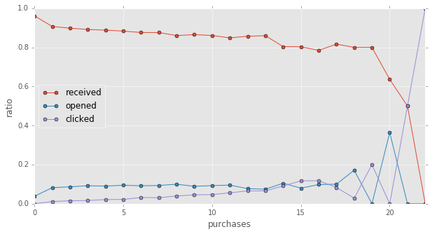

png

from above plot, we can know, the more items a certain user purchased previously, the more likely that user will open the email or click the link.

user’s country vs. response

grp_count_plotbar('country')

response	received	opened	clicked	total
country
ES	0.960570	0.031103	0.008327	9967.0
FR	0.958779	0.033217	0.008004	9995.0
UK	0.879282	0.096043	0.024675	19939.0
US	0.880481	0.095160	0.024360	60099.0

png

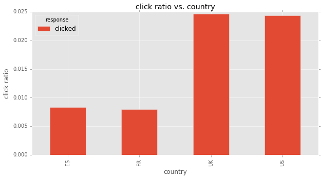
from above plots, we see that, ‘open percentage’ and ‘click percentage’ is much higher (nearly 3 times) in UK and US than in France and Spain.

this may be the translation issue. I guess the emails are written in English, which is unreadable to some non-English-speaking users, which cause the low ‘click ratio’ in non-English-speaking countries.

email’s version vs. response

grp_count_plotbar('is_personal')

response	received	opened	clicked	total
is_personal
0	0.920034	0.064829	0.015137	50209.0
1	0.871864	0.100842	0.027294	49791.0

png

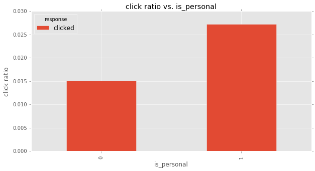
‘personalized email’ has higher ‘click ratio’ than ‘general email’. this is very easy to understand. Having my name in the recipient, at least I am some kind of ‘important’ to the company, other than some ordinary people which the company don’t bother to remember his name.

weekday vs. response

grp_count_plotbar('weekday')

response	received	opened	clicked	total
weekday
1	0.883590	0.093504	0.022906	14363.0
2	0.879092	0.096019	0.024889	14143.0
3	0.879296	0.093084	0.027620	14084.0
4	0.881348	0.094207	0.024445	14277.0
5	0.925019	0.060944	0.014037	14177.0
6	0.912005	0.070149	0.017846	14569.0
7	0.911448	0.071801	0.016751	14387.0

png

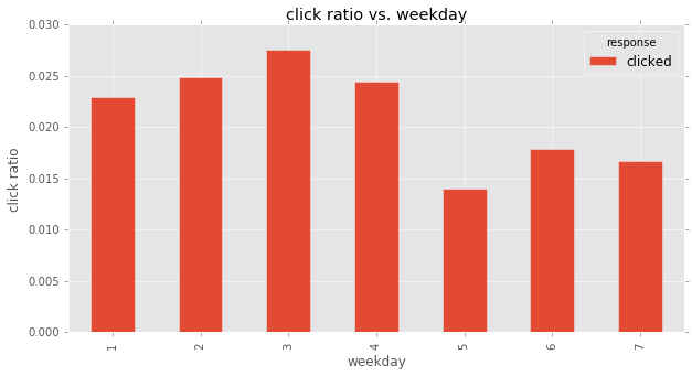
Friday, Saturday, Sunday have obviously lower ‘click ratio’ than Monday to Thursday. People normally don’t process emails during weekends.

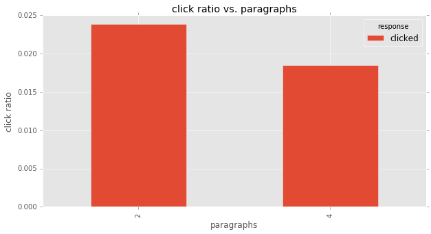
email text vs. response

grp_count_plotbar('paragraphs')

response	received	opened	clicked	total
paragraphs
2	0.883698	0.092430	0.023872	49724.0
4	0.908266	0.073196	0.018538	50276.0

png

sending hour vs. response

grp_count_plotbar('hour')

response	received	opened	clicked	total
hour
1	0.910840	0.071032	0.018128	2703.0
2	0.911589	0.072089	0.016322	3676.0
3	0.915184	0.065293	0.019523	4610.0
4	0.911419	0.072394	0.016186	5622.0
5	0.917417	0.064570	0.018013	6551.0
6	0.909176	0.073677	0.017147	7465.0
7	0.909434	0.072282	0.018284	8204.0
8	0.911407	0.069659	0.018933	8398.0
9	0.873725	0.100481	0.025794	8529.0
10	0.866993	0.104768	0.028240	8180.0
11	0.872645	0.100227	0.027128	7483.0
12	0.875230	0.099109	0.025661	6508.0
13	0.890521	0.089590	0.019889	5581.0
14	0.889520	0.089738	0.020742	4580.0
15	0.894074	0.081019	0.024907	3493.0
16	0.894165	0.082639	0.023197	2759.0
17	0.890650	0.090861	0.018489	1893.0
18	0.905700	0.078114	0.016186	1421.0
19	0.924862	0.058564	0.016575	905.0
20	0.911585	0.076220	0.012195	656.0
21	0.942466	0.049315	0.008219	365.0
22	0.931373	0.049020	0.019608	204.0
23	0.917241	0.041379	0.041379	145.0
24	0.840580	0.130435	0.028986	69.0

png

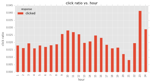
although from above plot, it seems ‘sending hour’ has some impact on ‘clicked ratio’. however, that may be caused by much fewer examples in late hours. also according to statistical test‘s result, I don’t think ‘sending hour’ is an important feature, and won’t include it in my model.

Answer question 4

Did you ﬁnd any interesting pattern on how the email campaign performed for diﬀerent segments of users? Explain.

from above explorary analysis, I can find some interesting patterns listed below:

The more item a certain user purchased in the past, the more likely that user will click the link
Users from English-speaking coutries are more likely to click the link, which may be caused by some translation issue.
Personalized email is more likely to be opened and clicked
Emails sent at weekends is less likely to be opened and clicked
Sending hour and #Paragraphs are not very important features to affect click rate

Build Predictive Model

In this section, I will build a model to predict whether a user will open the email and click the link inside it.

Prepare the data

del X
X = emails.copy()
X.sample(5)# get a feeling about current data

	hour	weekday	country	purchases	paragraphs	is_personal	response
email_id
785135	10	4	UK	4	4	0	received
479664	4	5	UK	0	4	0	received
233005	19	5	US	10	4	0	received
285041	15	2	US	7	4	1	received
10411	2	5	UK	5	4	0	received

# select original features
# 'paragraphs' isn't an important feature, but I will include it, and see how RF say about it
X = X.loc[:,["country","purchases","paragraphs","is_personal"] ]

# create new feature
X['is_weekend'] = (emails.weekday>=5).astype(int)

# One-Hot-Encode 'country' feature
X = pd.get_dummies(X,columns=["country"],drop_first=True)

# prepare the target
y = (emails.response == 'clicked').astype(int)

X.sample(5)# check the data

	purchases	paragraphs	is_personal	is_weekend	country_FR	country_UK	country_US
email_id
231912	5	2	1	1	0.0	0.0	0.0
538951	5	2	1	0	0.0	0.0	0.0
716309	5	2	1	0	1.0	0.0	0.0
695780	6	4	1	1	0.0	0.0	1.0
586318	2	4	1	0	0.0	0.0	1.0

# split for training and testing
Xtrain,Xtest,ytrain,ytest = train_test_split(X,y,test_size=0.33333,random_state = seed)

print 'Train set shape: {}, positive ratio={:.3f}'.format(Xtrain.shape,ytrain.mean())
print 'Test set shape: {}, positive ratio={:.3f}'.format(Xtest.shape,ytest.mean())

Train set shape: (66667, 7), positive ratio=0.021
Test set shape: (33333, 7), positive ratio=0.022

Train the model

Due to time limitation, I will just train one GBM model.

If given sufficient time, I will apply following strategies to improve the model:

build multiple models, and ensemble them (average or stacking) to improve the prediction performance.
try more hyper-parameters to find better ones.

train_matrix = xgb.DMatrix(Xtrain,ytrain)
test_matrix = xgb.DMatrix(Xtest)

params = {}
params['objective'] = 'binary:logistic'  # output probabilities
params['eval_metric'] = 'auc'
params["num_rounds"] = 300
params["early_stopping_rounds"] = 30
# params['min_child_weight'] = 2
params['max_depth'] = 6
params['eta'] = 0.1
params["subsample"] = 0.8
params["colsample_bytree"] = 0.8

cv_results = xgb.cv(params,train_matrix,
                    num_boost_round = params["num_rounds"],
                    nfold = params.get('nfold',5),
                    metrics = params['eval_metric'],
                    early_stopping_rounds = params["early_stopping_rounds"],
                    verbose_eval = True,
                    seed = seed)

[0]    train-auc:0.677493+0.00828721    test-auc:0.672627+0.00998874
[1]    train-auc:0.697782+0.00882727    test-auc:0.696658+0.0206434
[2]    train-auc:0.70463+0.00828662    test-auc:0.702561+0.0208773
[3]    train-auc:0.711914+0.00409068    test-auc:0.710696+0.0228788
[4]    train-auc:0.714488+0.00278646    test-auc:0.712043+0.0193185
[5]    train-auc:0.717649+0.00424529    test-auc:0.714465+0.0207032
[6]    train-auc:0.719344+0.00510737    test-auc:0.715544+0.0193956
[7]    train-auc:0.724209+0.00365824    test-auc:0.719632+0.0165027
[8]    train-auc:0.729045+0.00371847    test-auc:0.72386+0.0148701
[9]    train-auc:0.730501+0.00375046    test-auc:0.724429+0.0142755
[10]    train-auc:0.732467+0.0026696    test-auc:0.726337+0.0156743
[11]    train-auc:0.735537+0.00246068    test-auc:0.729132+0.0162888
[12]    train-auc:0.737188+0.00155158    test-auc:0.730848+0.0168706
[13]    train-auc:0.738333+0.00183292    test-auc:0.73156+0.016002
[14]    train-auc:0.740307+0.00175305    test-auc:0.732328+0.0157333
[15]    train-auc:0.741514+0.00256378    test-auc:0.733169+0.0154183
[16]    train-auc:0.742537+0.0021792    test-auc:0.733099+0.0151237
[17]    train-auc:0.744702+0.00246548    test-auc:0.735111+0.0143654
[18]    train-auc:0.744979+0.00216543    test-auc:0.735508+0.0144697
[19]    train-auc:0.746026+0.00214697    test-auc:0.736038+0.0145
[20]    train-auc:0.747204+0.00234766    test-auc:0.73719+0.0144764
[21]    train-auc:0.748409+0.0027355    test-auc:0.737671+0.0133952
[22]    train-auc:0.749618+0.00291407    test-auc:0.738383+0.0132849
[23]    train-auc:0.750261+0.0030989    test-auc:0.739096+0.0125292
[24]    train-auc:0.750758+0.00331821    test-auc:0.739578+0.0117813
[25]    train-auc:0.751382+0.00282425    test-auc:0.739345+0.0120623
[26]    train-auc:0.752415+0.00346696    test-auc:0.740137+0.010798
[27]    train-auc:0.75338+0.00363762    test-auc:0.740929+0.0106986
[28]    train-auc:0.754266+0.00323947    test-auc:0.741637+0.0107274
[29]    train-auc:0.754915+0.00302772    test-auc:0.741759+0.0112564
[30]    train-auc:0.755914+0.0028627    test-auc:0.742037+0.0113041
[31]    train-auc:0.756318+0.0033501    test-auc:0.7425+0.0109369
[32]    train-auc:0.756882+0.00331093    test-auc:0.74231+0.0109721
[33]    train-auc:0.757279+0.00329185    test-auc:0.742169+0.011238
[34]    train-auc:0.757727+0.00332192    test-auc:0.74215+0.0115881
[35]    train-auc:0.758015+0.00318842    test-auc:0.742415+0.0118561
[36]    train-auc:0.75832+0.00301207    test-auc:0.742148+0.0119087
[37]    train-auc:0.758837+0.00294787    test-auc:0.742522+0.0116916
[38]    train-auc:0.759134+0.00323002    test-auc:0.742998+0.0112852
[39]    train-auc:0.759435+0.00314337    test-auc:0.743453+0.0113958
[40]    train-auc:0.759625+0.00329416    test-auc:0.743103+0.0111658
[41]    train-auc:0.760182+0.00309855    test-auc:0.743537+0.0108819
[42]    train-auc:0.760478+0.00316004    test-auc:0.743372+0.011017
[43]    train-auc:0.760531+0.00324614    test-auc:0.743372+0.0112937
[44]    train-auc:0.760811+0.00309214    test-auc:0.743344+0.0112747
[45]    train-auc:0.761199+0.00302771    test-auc:0.743541+0.0114938
[46]    train-auc:0.761436+0.00302944    test-auc:0.743817+0.0118088
[47]    train-auc:0.761543+0.00314059    test-auc:0.744085+0.0117599
[48]    train-auc:0.761755+0.00306749    test-auc:0.744454+0.0118087
[49]    train-auc:0.761926+0.00314977    test-auc:0.744501+0.0118104
[50]    train-auc:0.762055+0.00309526    test-auc:0.744369+0.0119067
[51]    train-auc:0.762271+0.00292601    test-auc:0.744522+0.0120931
[52]    train-auc:0.762409+0.00301158    test-auc:0.744722+0.0119359
[53]    train-auc:0.762461+0.00298882    test-auc:0.744397+0.0117605
[54]    train-auc:0.762592+0.00298153    test-auc:0.744378+0.0119351
[55]    train-auc:0.762895+0.00297585    test-auc:0.744472+0.0118786
[56]    train-auc:0.762913+0.00296567    test-auc:0.744442+0.0117821
[57]    train-auc:0.763132+0.00301844    test-auc:0.744228+0.0117882
[58]    train-auc:0.763194+0.0029937    test-auc:0.744274+0.0116317
[59]    train-auc:0.763377+0.00302593    test-auc:0.744082+0.011701
[60]    train-auc:0.763542+0.00298474    test-auc:0.743952+0.0117522
[61]    train-auc:0.763706+0.00296295    test-auc:0.743824+0.0117634
[62]    train-auc:0.763734+0.00293909    test-auc:0.743966+0.0115998
[63]    train-auc:0.763867+0.00296588    test-auc:0.743936+0.0116863
[64]    train-auc:0.763986+0.0029833    test-auc:0.743937+0.0116513
[65]    train-auc:0.764118+0.00302993    test-auc:0.743966+0.0117081
[66]    train-auc:0.764343+0.00292955    test-auc:0.743819+0.01163
[67]    train-auc:0.76442+0.00289046    test-auc:0.743918+0.0116983
[68]    train-auc:0.76458+0.00284802    test-auc:0.744038+0.0113129
[69]    train-auc:0.764717+0.00293263    test-auc:0.743734+0.0113893
[70]    train-auc:0.764937+0.00289321    test-auc:0.743605+0.0114114
[71]    train-auc:0.764969+0.00291843    test-auc:0.743335+0.0114451
[72]    train-auc:0.765096+0.00293488    test-auc:0.743135+0.0116176
[73]    train-auc:0.765168+0.00292989    test-auc:0.743155+0.0116143
[74]    train-auc:0.765326+0.00296368    test-auc:0.743008+0.0114881
[75]    train-auc:0.765443+0.00296921    test-auc:0.743122+0.0115193
[76]    train-auc:0.765457+0.00295559    test-auc:0.743204+0.011375
[77]    train-auc:0.765536+0.00298759    test-auc:0.74318+0.0113059
[78]    train-auc:0.765807+0.00298637    test-auc:0.74306+0.0113673
[79]    train-auc:0.765864+0.00301058    test-auc:0.743087+0.0114866
[80]    train-auc:0.765975+0.00306381    test-auc:0.743178+0.011708
[81]    train-auc:0.766011+0.00310261    test-auc:0.743395+0.0116618

n_best_trees = cv_results.shape[0]
print "best number of trees: {}".format(n_best_trees)

best number of trees: 53

watchlist = [(train_matrix, 'train')]
gbt = xgb.train(params, train_matrix, n_best_trees,watchlist)

[0]    train-auc:0.702188
[1]    train-auc:0.704781
[2]    train-auc:0.71018
[3]    train-auc:0.714805
[4]    train-auc:0.715547
[5]    train-auc:0.726005
[6]    train-auc:0.725821
[7]    train-auc:0.725022
[8]    train-auc:0.7335
[9]    train-auc:0.735223
[10]    train-auc:0.736723
[11]    train-auc:0.74205
[12]    train-auc:0.742289
[13]    train-auc:0.742862
[14]    train-auc:0.743885
[15]    train-auc:0.743699
[16]    train-auc:0.742109
[17]    train-auc:0.744295
[18]    train-auc:0.746087
[19]    train-auc:0.74534
[20]    train-auc:0.743896
[21]    train-auc:0.74842
[22]    train-auc:0.7502
[23]    train-auc:0.750863
[24]    train-auc:0.750096
[25]    train-auc:0.752116
[26]    train-auc:0.752202
[27]    train-auc:0.752974
[28]    train-auc:0.752529
[29]    train-auc:0.752424
[30]    train-auc:0.753932
[31]    train-auc:0.753449
[32]    train-auc:0.754669
[33]    train-auc:0.755053
[34]    train-auc:0.755589
[35]    train-auc:0.755971
[36]    train-auc:0.757188
[37]    train-auc:0.757529
[38]    train-auc:0.757631
[39]    train-auc:0.757584
[40]    train-auc:0.757568
[41]    train-auc:0.758382
[42]    train-auc:0.758155
[43]    train-auc:0.758213
[44]    train-auc:0.758067
[45]    train-auc:0.7586
[46]    train-auc:0.758911
[47]    train-auc:0.759027
[48]    train-auc:0.759092
[49]    train-auc:0.759198
[50]    train-auc:0.759484
[51]    train-auc:0.759869
[52]    train-auc:0.760239

# plot feature importances
xgb.plot_importance(gbt)

<matplotlib.axes._subplots.AxesSubplot at 0x11ffb4e90>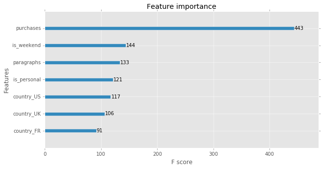

png

above feature importance match the result from explorary analysis.

Plot ROC curve and choose better probability threshold

since the data is highly imbalanced (positive examples is only 2% of the total examples), if using default probability threshold (0.5), the model just classify every example as negative, so we need to plot the ROC curve and choose a better probability threshold.

But ROC cannot be plot on either training set or test set. so I split the original train set into ‘training’ and ‘validation’ sets, re-train on ‘training set’ and plot ROC on ‘validation set’.

print "n_best_trees={},xgboost parameters: ".format(n_best_trees)
params

n_best_trees=53,xgboost parameters: 





{'colsample_bytree': 0.8,
 'early_stopping_rounds': 30,
 'eta': 0.1,
 'eval_metric': 'auc',
 'max_depth': 6,
 'num_rounds': 300,
 'objective': 'binary:logistic',
 'subsample': 0.8}

# define a function, avoid pollute the current namespace
def validation_roc():
    Xtrain_only,Xvalid,ytrain_only,yvalid = train_test_split(Xtrain,ytrain,test_size=0.2,random_state=seed)

    train_only_matrix = xgb.DMatrix(Xtrain_only,ytrain_only)
    valid_matrix = xgb.DMatrix(Xvalid)

    # retrain on training set
    gbt_train_only = xgb.train(params, train_only_matrix, n_best_trees)

    # predict on validation set
    yvalid_probas = gbt_train_only.predict(valid_matrix, ntree_limit=n_best_trees)

    d = {}
    d['FPR'],d['TPR'],d['Threshold'] = roc_curve(yvalid,yvalid_probas)
    return pd.DataFrame(d)

roc_results = validation_roc()

_ = plt.figure()
plt.plot(roc_results.FPR,roc_results.TPR)
plt.xlabel("FPR")
plt.ylabel('TPR')

<matplotlib.text.Text at 0x11abea2d0>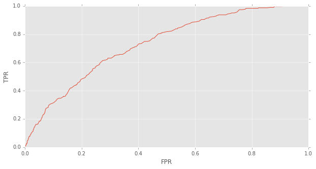

png

according to above ROC curve and make a compromise between Precision and Recall, I decide to choose a threshold which makes TPR at about 0.6, then FPR will be about 0.3, which I think is acceptable.

roc_results.loc[(roc_results.TPR > 0.6) & (roc_results.TPR < 0.65),:]

	FPR	TPR	Threshold
192	0.274192	0.613861	0.030303
193	0.274729	0.613861	0.030261
194	0.274960	0.613861	0.030247
195	0.284245	0.617162	0.030224
196	0.288389	0.620462	0.029755
197	0.288619	0.620462	0.029587
198	0.290998	0.623762	0.029482
199	0.291229	0.623762	0.029463
200	0.291996	0.630363	0.029195
201	0.292380	0.630363	0.029118
202	0.294298	0.630363	0.028849
203	0.295296	0.630363	0.028624
204	0.296217	0.630363	0.028613
205	0.302663	0.630363	0.028445
206	0.303661	0.630363	0.028363
207	0.303737	0.630363	0.028344
208	0.304044	0.630363	0.028225
209	0.313944	0.643564	0.028042
210	0.314020	0.646865	0.028016
211	0.315709	0.646865	0.027908
212	0.316016	0.646865	0.027625

# choose a threshold based on ROC
# FPR=0.292380, TPR=0.630363, Threshold=0.029118
pos_prob_threshold = 0.029118

def adjust_predict(matrix):
    y_probas = gbt.predict(matrix, ntree_limit=n_best_trees)
    return (y_probas > pos_prob_threshold).astype(int)

ytrain_pred = adjust_predict(train_matrix)
print classification_report(ytrain,ytrain_pred)

             precision    recall  f1-score   support

          0       0.99      0.72      0.83     65265
          1       0.05      0.65      0.09      1402

avg / total       0.97      0.71      0.82     66667

ytest_pred = adjust_predict(test_matrix)
print classification_report(ytest,ytest_pred)

             precision    recall  f1-score   support

          0       0.99      0.71      0.83     32616
          1       0.04      0.60      0.08       717

avg / total       0.97      0.71      0.81     33333

more accurate Precision and Recall

print "test precision: {:.2f}%".format(precision_score(ytest,ytest_pred) * 100)
print "test recall: {:.2f}%".format(recall_score(ytest,ytest_pred) * 100)

test precision: 4.35%
test recall: 60.11%

gbt.save_model('gbt.model')

Answer question 2 and question 3’s first part

The VP of marketing thinks that it is stupid to send emails to a random subset and in a random way. Based on all the information you have about the emails that were sent, can you build a model to optimize in future email campaigns to maximize the probability of users clicking on the link inside the email?
By how much do you think your model would improve click through rate ( deﬁned as # of users who click on the link / total users who received the email). How would you test that?

I have build a Gradient Boosting Tree model in previous section which predicts whether a user will click the link or not. Then the new email campaign strategy will be: only send email to users which my GBM model predicts positive.

n_emails_old_sent = ytest_pred.shape[0]
n_emails_new_sent = ytest_pred.sum()
saving_percentage = 100 - n_emails_new_sent * 100.0/n_emails_old_sent
pd.Series({'#emails sent in old way': n_emails_old_sent,
           '#emails sent in new way': n_emails_new_sent,
           'saving percentage (%)': saving_percentage})

#emails sent in new way     9904.000000
#emails sent in old way    33333.000000
saving percentage (%)         70.287703
dtype: float64

according to its predictive result on test set

my model only need to send 30% of the old email amount, saving 70% amount.
my model will cover 60% of valued users which will click the link.
4.35% of the receiver will open email and click the link. compare with old strategy, whose click rate is 2.12% , my new strategy can double the click rate.

Answer question 3’s second part

By how much do you think your model would improve click through rate ( deﬁned as # of users who click on the link / total users who received the email). How would you test that?

To test my conclusion, we need to perform a A/B test:

randomly assign users to two groups, Control group and Experiment group.
in Control group, still use the old email-campaign strategy, i.e., just send emails to all users in Control group.
in Experiment group, use my model to predict whether the user will click the link or not. and only send emails to those users whose predictive result is positive.
then we preform a one-tail unpaired t-test to test whether Experiement group’s population proportion is higher than Control group’s population proportion.

ISLR_ch3.1 Simple Linear Regression

ISLR_ch3.1 Simple Linear RegressionSimple linear regression: approach for predicting a quantitative response Y on the ba

2019-09-23 An Introduction to statistical Learning

Machine Learning notes

6-Price Test

Background: This notebook aims to evaluate whether a pricing test running on the site has been successful. Specifically,

2018-01-31 Take home data challenge

Python_Take home challenge